
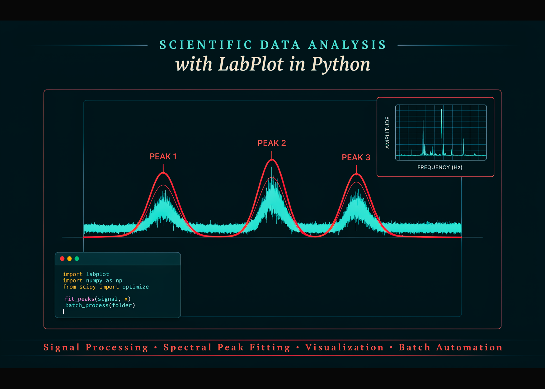
In this tutorial, we explore aLabPlot-inspired scientific data analysis workflow in Python while preserving the structure and terminology of LabPlot’s aspect tree, analysis kernels, plotting system, and project model. We build reusable components to import tabular data, compute descriptive statistics, smooth and differentiate signals, perform Fourier analysis and filtering, detect peaks, integrate curves, reduce data, and fit nonlinear models with detailed statistical diagnostics. We then apply these tools to a realistic spectroscopy example: removing periodic interference, identifying overlapping peaks, fitting a multi-Gaussian model, inspecting residuals, visualizing results through themed worksheets, exporting figures, and saving project data in LabPlot-compatible .lml-style files. Finally, we extend the same workflow to batch processing so we can analyze multiple temperature-dependent spectra and fit secondary trends across the resulting measurements.
We set up the Python environment, configure reproducibility, and establish the output directory for the tutorial. We recreate LabPlot’s core aspect-tree structure using projects, spreadsheets, columns, plot designations, and column modes. We also implement the AsciiFilter workflow to import structured text data into our LabPlot-style data model.
We implement the main numerical analysis kernels that let us smooth, differentiate, integrate, transform, filter, reduce, and inspect scientific signals. We add peak detection along with Gaussian and Lorentzian models for advanced curve analysis. We also build nonlinear fitting utilities that calculate parameter uncertainties, confidence intervals, goodness-of-fit statistics, and maximum-likelihood distribution fits.
We construct the visualization layer using curves, histograms, Cartesian plots, worksheets, themes, and reusable analysis-curve objects. We connect these plotting objects directly to our numerical operations so we can recalculate processed curves and fitted models programmatically. We also implement LabPlot-style project file loading and saving, including compressed .lml formats and spreadsheet reconstruction.
We generate a realistic noisy spectroscopy dataset containing a sloping baseline, overlapping Gaussian peaks, periodic interference, and random noise. We use Fourier analysis, band-reject filtering, smoothing, differentiation, and peak detection to isolate key spectral features before fitting. We then perform a constrained multi-Gaussian fit, integrate the recovered signal, reduce the data, calculate a Hilbert envelope, and statistically evaluate the fit residuals.
Kami mengatur hasil spektroskopi ke dalam lembar kerja bertema yang berisi spektrum mentah, komponen yang dipasang, spektrum Fourier, puncak yang terdeteksi, dan distribusi residu. Kami mengekspor visualisasi lengkap ke format PNG, PDF, dan SVG sehingga kami memiliki keluaran grafis yang dapat digunakan kembali. Kami juga menyimpan pengukuran yang telah diproses dan parameter yang dipasang di dalam proyek, menyimpannya dalam beberapa format .lml, dan memverifikasi bahwa data proyek bertahan sepanjang perjalanan.
Kami memperluas alur kerja dari satu spektrum ke kumpulan pengukuran sintetis yang bergantung pada suhu dan secara otomatis menganalisis setiap file. Kami mengekstrak area dan pusat puncak yang dipasang, melakukan kecocokan eksponensial sekunder, memvisualisasikan ketergantungan suhu, dan mengukur penyimpangan spektral yang dipulihkan. Kami akhirnya menghubungkan alur kerja yang kami emulasi ke konsep pylabplot SDK yang setara dan mencantumkan keluaran tutorial yang dihasilkan.
Sebagai kesimpulan, kami membangun alur analisis ilmiah lengkap yang mencerminkan banyak konsep inti LabPlot sekaligus memungkinkan kami menjalankan alur kerja secara langsung dengan Python. Kami beralih dari impor data terstruktur dan inspeksi statistik ke pemrosesan sinyal, pemfilteran domain Fourier, deteksi puncak, pemasangan multi-puncak nonlinier, integrasi, analisis residu, visualisasi, serialisasi proyek, dan pemrosesan batch otomatis. Dengan menggabungkan tahapan-tahapan ini, kita dapat mengubah pengukuran eksperimental yang berisik menjadi parameter yang dapat diinterpretasikan, plot yang siap dipublikasikan, keluaran proyek yang dapat digunakan kembali, dan tren tingkat yang lebih tinggi seperti perilaku puncak yang bergantung pada suhu. Kami juga membangun jembatan praktis antara implementasi Python dan pylabplot SDK yang sebenarnya, memberi kami landasan untuk mentransfer alur kerja yang sama ke lingkungan LabPlot asli.
Lihat KODE LENGKAP di sini. Juga, jangan ragu untuk mengikuti kami di Twitter dan jangan lupa untuk bergabung dengan SubReddit 150rb+ML kami dan Berlangganan Buletin kami. Tunggu! apakah kamu aktif?